toc: true layout: post description: Image processing with OpenCV categories: [learning] comments: true

title: "Image processing with OpenCV: Part 1"

Image processing with OpenCV: Part 1

Disclaimer

The notebook is prepared on initial repo: https://github.com/MakarovArtyom/OpenCV-Python-practices

Acknowledgement

The code from Jupyter notebooks follows Udacity Computer Vision nanodegree logic.
More Computer Vision exercises can be found under Udacity CVND repo: https://github.com/udacity/CVND_Exercises

Libraries

# uncomment in case PyQt5 is not installed
#! pip install PyQt5

import numpy as np
import matplotlib.pyplot as plt
# for image reading
import matplotlib.image as mpimg
import cv2

# makes image pop-up in interactive window
%matplotlib qt

Image reading

Given an RGB image, let's read it using matplotlib (mpimg) .

The RGB color model is an additive color model in which red, green, and blue light are added together in various ways to reproduce a broad array of colors. The name of the model comes from the initials of the three additive primary colors, red, green, and blue

Source: https://en.wikipedia.org/wiki/RGB_color_model

image = mpimg.imread('images/robot_blue.jpg')

print('Shape of the image:', image.shape)

Shape of the image: (720, 1280, 3)

Per single image, we can retrieve the following info:

• height = 720
• width = 1280
• number of channels = 3

Later on, we will see that for many "classical" computer vision algorithms the color information is redundant.
For solving problems like edge, corner or blob detection, the grayscale image is enough.

Let's use cvtColor function to convert RGB image to gray.

gray_img = cv2.cvtColor(image, cv2.COLOR_RGB2GRAY)
plt.imshow(gray_img, cmap = 'gray')

<matplotlib.image.AxesImage at 0x7fdd7c819828>


print('Shape of the image after convertation:', gray_img.shape)

Shape of the image after convertation: (720, 1280)

It's important to understand an image is just a matrix (tensor) with values, representing the intensity of pixels (from 0 to 255).
Each pixel has it's own coordinates.

print('Max pixel value:', gray_img.max())
print('Min pixel value:', gray_img.min())

Max pixel value: 255
Min pixel value: 0

Use the pair of (x,y) coordinates to access particular pixel's value.

x = 45
y = 52

pixel_value = gray_img[x,y]
print(pixel_value)

28

Note, it's possible to manipulate pixel values by scalar multiplication and augmentation in different formats.

Example: let's create a 6x6 image with random pixel values.

pixel = abs(np.random.randn(6,6)) * 10
pixel.astype(int)

array([[15,  8,  3, 14,  3,  3],
       [ 6,  9, 10,  7,  0,  5],
       [11, 18, 10,  4, 14,  5],
       [ 9,  6,  0,  1,  1, 16],
       [18,  9,  6, 29,  8,  7],
       [12,  0,  2,  0,  9, 12]])

Next, display the results with grayscale colormap.

plt.matshow(pixel, cmap = 'gray')

<matplotlib.image.AxesImage at 0x7fdd7acd96d8>

Color isolating

%matplotlib inline

Let's read an image and see how we can visualize 3 RBG colors individually.

img = mpimg.imread('images/car.jpeg')
plt.imshow(img)

<matplotlib.image.AxesImage at 0x7feaec8de0b8>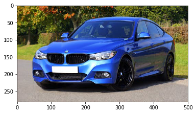


print('Shape of the image:', img.shape)

Shape of the image: (281, 500, 3)

Since the color image is a tensor composed of 3 colors, we can express "red", "green" and "bleu" as follows.

r = img[:,:, 0] # red
g = img[:,:, 1] # green
b = img[:,:, 2] # blue
print('Shape of individual color matrix:', r.shape)

Shape of individual color matrix: (281, 500)

f, (ax1, ax2, ax3) = plt.subplots(1,3, figsize=(20,10))

# visualize red
ax1.set_title('R channel')
ax1.imshow(r, cmap = 'gray')
# green
ax2.set_title('G channel')
ax2.imshow(g, cmap = 'gray')
# blue
ax3.set_title('B channel')
ax3.imshow(b, cmap = 'gray')

<matplotlib.image.AxesImage at 0x7feb0295d550>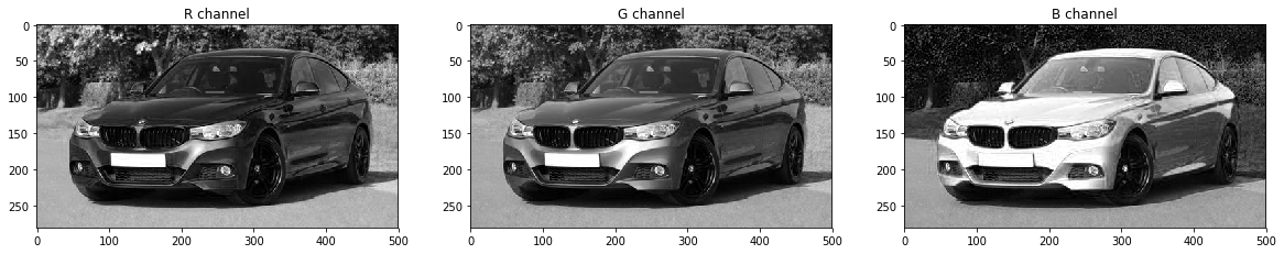


Background change

Isolating object's background

Additional resources:

• Color picker to choose boundaries: https://www.w3schools.com/colors/colors_picker.asp

Suppose we have an image of an object on solid color background.
Consider the image of a robot below - we read it with open-cv library.

img = cv2.imread('images/robot_blue.jpg')
plt.imshow(img)

<matplotlib.image.AxesImage at 0x7feaec56f6d8>

Important note: open-cv reads images as BGR, not RGB - as a result the output is different from original image.
In particular - red and blue colors are in reverse order.

Next, we take a copy of image and change it from BGR to RGB (pass parameter cv2.COLOR_BGR2RGB).
Note, that any transformations applied to a copy will not effect an image.

"""
- make a copy with numpy
- change from BGR to RGB
"""

img_copy = np.copy(img)

img_copy = cv2.cvtColor(img_copy, cv2.COLOR_BGR2RGB)
plt.imshow(img_copy)

<matplotlib.image.AxesImage at 0x7feaec6dc4e0>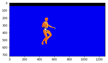


First, define color a threshold. It will be a lower and upper bounds for the background I wnat to isolate.
Here we need to specify 3 values - for each color - red, green and blue.

• Lower bound: red and green as zero, and high value for blue. For example, 230.
  
• Upper bound: red, green - some small values and blue - maximum, i.e. 250. So, allow a bit red and green.
  

All values within this range will be considered as intense blue color. This range will be replaced by another background.

blue_lower = np.array([0, 0, 230])
blue_upper = np.array([50, 50, 250])

Creating mask

We are going to use a common way to isolate chosen area - creating a mask.
Now, we will isolate blue background area using inRange() function.
It verifies each pixel whether it falls into specific range, defined by lower and upper bounds.

• If it falls - the white mask will be displayed;
• If it does not fall within the range - pixel will be turned into black.

Simply saying, everything inside the interval will be white.

"""
- function will take lower and upper bounds of image
- and define the mask
"""
mask = cv2.inRange(img_copy, blue_lower, blue_upper)
plt.imshow(mask, cmap = 'gray')

<matplotlib.image.AxesImage at 0x7feaec74afd0>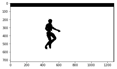


• White area - area, where the new image background will be displayed.
• Black area - where ew image background will be blocked out.

The mask has the same height and width, and each pixel has 2 values:

• 255 - for white area;
• 0 - for black area.

Now, let's put our object into a mask.

• First of all, create a copy of image (just if we want to change it later on).
  
• Then, one way to separate blue background from this is to check where blue pixels intersect with mask white pixels, or in other words - do not intersect with black (not equal 0).
  We will set them to black color.

Displaying an image, we will see that only object appears on a black background.

masked_img = np.copy(img_copy)
masked_img[mask!=0] = [0,0,0]

plt.imshow(masked_img)

<matplotlib.image.AxesImage at 0x7feaec47eba8>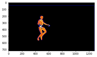


Applying new background

Next step will be just to apply new background on top of black one.
We just take an image, (e.g. "space image" below and convert it from BGR to RGB).

background_img = cv2.imread('images/background_img.jpg')
background_img = cv2.cvtColor(background_img, cv2.COLOR_BGR2RGB)
plt.imshow(background_img)

<matplotlib.image.AxesImage at 0x7feaec4e4630>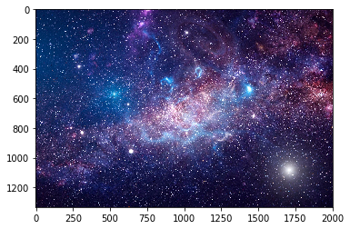


It's also important to crop background image to make it the same size as our robot image. We crop it by height and width.

"""
- cropping to a size of (720, 1280)
"""

crop_background_img = background_img[0:720, 0:1280]

Now, we will do an opposite operation with a cropped background image: choose pixels that are equal to 0 in mask image (there we had black robot) and set these pixels to a black on cropped background image.

Simply saying, we merge mask and crop_background_img.

crop_background_img[mask == 0] = [0,0,0]
plt.imshow(crop_background_img)

<matplotlib.image.AxesImage at 0x7feaeb3c8278>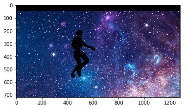


Final step: add object and new background together

Since the black area on cropped background image is equivalent to 0, we can add this image to masked image.
In this case simple summation will work, since we deal with matrices.

final_image = crop_background_img + masked_img
plt.imshow(final_image)

<matplotlib.image.AxesImage at 0x7feaeb425be0>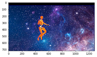


Object detection in HSV space

HSV colorspace

HSV colorspace is similar to RGB and also represents 3 channel - hue, saturation and value.
This space is commonly used in tasks like image segmentation.
In HSV colorspace Hue channel models color type, while Saturation and Value represents color as a mixture of shades and brightness.

Since the hue channel models the color type, it is very useful in image processing tasks that need to segment objects based on its color. Variation of the saturation goes from unsaturated to represent shades of gray and fully saturated (no white component). Value channel describes the brightness or the intensity of the color.

Source: https://docs.opencv.org/3.4/da/d97/tutorial_threshold_inRange.html

We will start with image displaying. We will use both RGB and HSV color spaces to detect the balloons in the image.

img = cv2.imread('images/baloons.jpg')
img_copy = np.copy(img)

img_copy = cv2.cvtColor(img_copy, cv2.COLOR_BGR2RGB)
plt.imshow(img_copy)

<matplotlib.image.AxesImage at 0x7feaef450a58>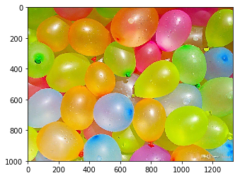


First, let's plot the color channels in RGB space.

# RGB channels
# we take all pixels, but isolate the color we need

red = img_copy[:,:,0]
green = img_copy[:,:,1]
blue = img_copy[:,:,2]

# now, plot each of this colors in gray scale to see the relative intensities
f, (ax1, ax2, ax3) = plt.subplots(1,3, figsize = (20,10))

ax1.set_title('Red scale')
ax1.imshow(red, cmap = 'gray')

ax2.set_title('Green scale')
ax2.imshow(green, cmap = 'gray')

ax3.set_title('Blue scale')
ax3.imshow(blue, cmap = 'gray')

<matplotlib.image.AxesImage at 0x7feaefa82630>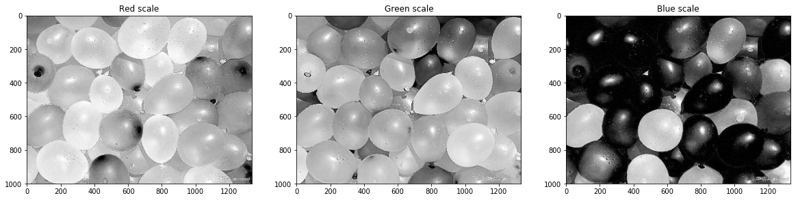


We can see that pink balloons have high values for the red (close to 255, white color) and medium values for blue.
However, there are many variations, especially if the balloon is in shadow.

Next, we convert image from RGB to HSV.

hsv = cv2.cvtColor(img_copy, cv2.COLOR_RGB2HSV)

Now, we isolate each of these channels as we did before.

hue = hsv[:,:,0]
saturation = hsv[:,:,1]
value = hsv[:,:,2]


f, (ax1, ax2, ax3) = plt.subplots(1,3, figsize = (20,10))
ax1.set_title('Hue')
ax1.imshow(hue, cmap = 'gray')

ax2.set_title('Saturation')
ax2.imshow(saturation, cmap = 'gray')

ax3.set_title('Value')
ax3.imshow(value, cmap = 'gray')

<matplotlib.image.AxesImage at 0x7feaf0b542b0>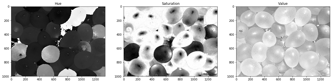


Compare this to our image. Take a look at pink balloons:

• Hue has high values for pink balloons, and even in shadow hue level is pretty consistent;
• Saturation values are quite versatile depending on shadow.

Create thresholds for pink color in RGB and HSV

Now, create lower and upper bounds for pink color in RGB and then in HSV spaces.

# use thrashold for pink color in RGB
# link to check: https://www.w3schools.com/colors/colors_rgb.asp

lower_pink = np.array([180,0,100])
upper_pink = np.array([255,255,230])

Then, do the same for HSV.
Remember, that hue goes from 0 to 180 degrees. We will limit this from 160 to 180.
Will allow any values for saturation and value from 0 to 255.

lower_hue = np.array([140,0,0])
upper_hue = np.array([180,255,255])

Mask the images

Now, we will create a mask to see how well these thresholds select the pink balloons.
As previous we will use inRage() function and apply mask afterwards.

"""
- first we create mask based on lower and upper bounds. Mask will assign 0 to all pixels that are out of these interval.
- then we make all pixels, intersecting with black color (have 0 values) black (assign to [0,0,0]).
- isolate pink color
"""

mask_rgb = cv2.inRange(img_copy, lower_pink, upper_pink)
masked_image = np.copy(img_copy)
masked_image[mask_rgb == 0] = [0,0,0]

plt.imshow(masked_image)
plt.title('RGB selection')

Text(0.5, 1.0, 'RGB selection')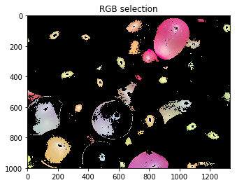


Here we can see RGB colorspace:

• Does not select all pink balloons (or ones that are in shadow);
• Selects some other colors.

Finally, repeat the procedure for HSV colorspace.

"""
 - note, we will use hsv image (RGB2HSV)
"""
mask_hsv = cv2.inRange( hsv, lower_hue, upper_hue)
masked_image = np.copy(hsv)
masked_image[mask_hsv == 0] = [0,0,0]

plt.imshow(masked_image)
plt.title('HSV selection')

Text(0.5, 1.0, 'HSV selection')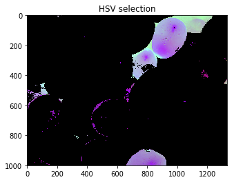


Day and Night Image Classifier

The day/night image dataset consists of 200 RGB color images in two categories: day and night. There are equal numbers of each example: 100 day images and 100 night images.

We'd like to build a classifier that can accurately label these images as day or night, and that relies on finding distinguishing features between the two types of images!

Note: All images come from the AMOS dataset (Archive of Many Outdoor Scenes).

Training and Testing Data

The 200 day/night images are separated into training and testing datasets.

• 60% of these images are training images, for you to use as you create a classifier.
• 40% are test images, which will be used to test the accuracy of your classifier.

First, we set some variables to keep track of some where our images are stored:

`image_dir_training`: the directory where our training image data is stored
`image_dir_test`: the directory where our test image data is stored

# Image data directories
image_dir_training = "training"
image_dir_test = "test"

Load the datasets

These first few lines of code will load the training day/night images and store all of them in a variable, IMAGE_LIST. This list contains the images and their associated label ("day" or "night").

For example, the first image-label pair in IMAGE_LIST can be accessed by index:

```python
# Using the load_dataset function in helpers.py
# Load training data
IMAGE_LIST = helpers.load_dataset(image_dir_training)

Train dataset contains:

• Images, classified as "day" or "night";
• It's possible to access first pair "image-label" by index 0 - IMAGE_LIST[0]
• To access label of e.g. first image - IMAGE_LIST[0][0].

Visualize the input images

First, lets select an image and its label, print the shape.

# Select an image and its label by list index
image_index = 0
selected_image = IMAGE_LIST[image_index][0]
selected_label = IMAGE_LIST[image_index][1]

print(selected_image.shape)
print(selected_label)

(458, 800, 3)
day

Display day and night images and check the difference between them.

# start with day image
# convert it to RGB format

selected_copy = np.copy(IMAGE_LIST[image_index][0])
selected_copy = cv2.cvtColor(selected_copy, cv2.COLOR_BGR2RGB)
plt.imshow(selected_copy, cmap = 'gray')
plt.title(IMAGE_LIST[image_index][1])

Text(0.5, 1.0, 'day')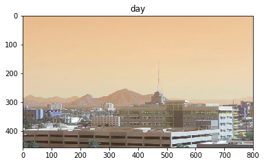


# Select an image and its label by list index
image_index = 43
night_image = IMAGE_LIST[image_index][0]
night_label = IMAGE_LIST[image_index][1]

print(night_image.shape)
print(night_label)

(458, 800, 3)
night

# pursue with night image
# convert it to RGB format

night_copy = np.copy(IMAGE_LIST[image_index][0])
night_copy = cv2.cvtColor(night_copy, cv2.COLOR_BGR2RGB)
plt.imshow(night_copy, cmap = 'gray')
plt.title(IMAGE_LIST[image_index][1])

Text(0.5, 1.0, 'night')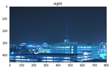


Standardize images

Let's create a class for input standartization.
Note, we need to standardize 2 objects:

• image;
• its label (convert categorical to numerical).

We will:

• resize image with shape (600x1100 px);
• convert day to 1 and night to 0;
• output a list of standardized images.

class Standardize():
    def __init__(self):
        # self.image_list = image_list
        self.standardized_list = []
        self.numerical_value = 0

    # initialize the function
    def standardize_input(self, image_list):
        for item in image_list:
            # image has index 0
            # label has index 1
            image = item[0]
            label = item[1]
            image = np.copy(image)
            label = np.copy(label)
            # start with image resize
            image_std = cv2.resize(image, (1100, 600))
            label_binary = self.numerical_value if label == 'night' else 1
            self.standardized_list.append((image_std, label_binary))
        return self.standardized_list

s1 = Standardize()
IMAGE_LIST_stand = s1.standardize_input(IMAGE_LIST)

print("Length of standardized images dataset:",len(IMAGE_LIST_stand))
print("Length of original images dataset:",len(IMAGE_LIST))

Length of standardized images dataset: 79
Length of original images dataset: 79

example_img = IMAGE_LIST_stand[0][0]
example_img = np.copy(example_img)

plt.imshow(example_img)
print('Image label:', IMAGE_LIST_stand[0][1])

Image label: 1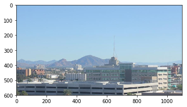


Feature extraction

Now, we are ready to separate these images on day and night based on average brightness.
This will be a single value and we assume, that average value for day will be higher than average value for night.
To calculate average brightness we will use HSV colorspace - Value channel in particular: we will sum it up and divide by area of image (height multiplied by width).

First of all, we will take a look at couple of day and night images.
Lets convert them from RGB to HSV.

# fist day image
# use standardized list of images we prepared above
img_day_1 = IMAGE_LIST_stand[0][0]
img_day_1 = np.array(img_day_1)
img_day_1 = cv2.cvtColor(img_day_1, cv2.COLOR_RGB2HSV)

# second day image
img_day_2 = IMAGE_LIST_stand[1][0]
img_day_2 = np.array(img_day_2)
img_day_2 = cv2.cvtColor(img_day_2, cv2.COLOR_RGB2HSV)

# fist night image
img_night_1 = IMAGE_LIST_stand[43][0]
img_night_1 = np.array(img_night_1)
img_night_1 = cv2.cvtColor(img_night_1, cv2.COLOR_RGB2HSV)

# second night image
img_night_2 = IMAGE_LIST_stand[53][0]
img_night_2 = np.array(img_night_2)
img_night_2 = cv2.cvtColor(img_night_2, cv2.COLOR_RGB2HSV)

Below we display day and night images in HSV colorspace.

image_day_1_h = img_day_1[:,:,0]
image_day_1_s = img_day_1[:,:,1]
image_day_1_v = img_day_1[:,:,2]

fig, (ax0, ax1,ax2,ax3) = plt.subplots(1,4, figsize = (20,10))

ax0.imshow(IMAGE_LIST_stand[0][0])
ax0.set_title('Standardized day image 1')
ax1.imshow(image_day_1_h, cmap = 'gray')
ax1.set_title('Hue, day image 1')
ax2.imshow(image_day_1_s, cmap = 'gray')
ax2.set_title('Saturation, day image 1')
ax3.imshow(image_day_1_v, cmap = 'gray')
ax3.set_title('Value, day image 1')

Text(0.5, 1.0, 'Value, day image 1')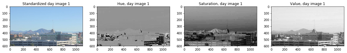


image_day_2_h = img_day_2[:,:,0]
image_day_2_s = img_day_2[:,:,1]
image_day_2_v = img_day_2[:,:,2]

fig, (ax0, ax1,ax2,ax3) = plt.subplots(1,4, figsize = (20,10))
ax0.imshow(IMAGE_LIST_stand[1][0])
ax0.set_title('Standardized day image 2')
ax1.imshow(image_day_2_h, cmap = 'gray')
ax1.set_title('Hue, image 2')
ax2.imshow(image_day_2_s, cmap = 'gray')
ax2.set_title('Saturation, image 2')
ax3.imshow(image_day_2_v, cmap = 'gray')
ax3.set_title('Value, image 2')

Text(0.5, 1.0, 'Value, image 2')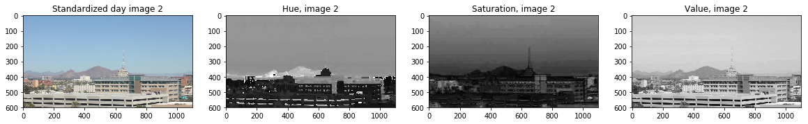


Based on days images we can say, that Value channel is high for the skies.

img_night_1_h = img_night_1[:,:,0]
img_night_1_s = img_night_1[:,:,1]
img_night_1_v = img_night_1[:,:,2]

fig, (ax0, ax1,ax2,ax3) = plt.subplots(1,4, figsize = (20,10))

ax0.imshow(IMAGE_LIST_stand[43][0])
ax0.set_title('Standardized night image 1')
ax1.imshow(img_night_1_h, cmap = 'gray')
ax1.set_title('Hue, night image 1')
ax2.imshow(img_night_1_s, cmap = 'gray')
ax2.set_title('Saturation, night  image 1')
ax3.imshow(img_night_1_v, cmap = 'gray')
ax3.set_title('Value, night image 1')

Text(0.5, 1.0, 'Value, night image 1')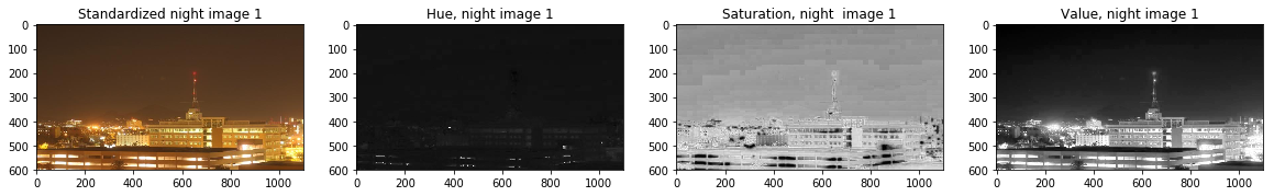


img_night_2_h = img_night_2[:,:,0]
img_night_2_s = img_night_2[:,:,1]
img_night_2_v = img_night_2[:,:,2]

fig, (ax0, ax1,ax2,ax3) = plt.subplots(1,4, figsize = (20,10))

ax0.imshow(IMAGE_LIST_stand[53][0])
ax0.set_title('Standardized night image 2')
ax1.imshow(img_night_2_h, cmap = 'gray')
ax1.set_title('Hue, night image 2')
ax2.imshow(img_night_2_s, cmap = 'gray')
ax2.set_title('Saturation, night  image 2')
ax3.imshow(img_night_2_v, cmap = 'gray')
ax3.set_title('Value, night image 2')

Text(0.5, 1.0, 'Value, night image 2')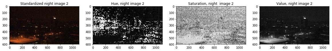


Find average brightness using V channel

Write the class that inputs entire list of standardized images and outputs following:

• new list with added average brightness to tuple: pair of image, label;
• visulalize distribution of night and day averages.

plt.style.use('ggplot')
%matplotlib inline

class AverageBrightness():

    def __init__(self):
        # define two functions: add value to pair
        # and visualize distributions
        self.list_with_bright = []
        self.night_list = []
        self.day_list = []
    def average_bright(self, standardized_list):
        for item in standardized_list:
            rgb_image = item[0]
            hsv = cv2.cvtColor(rgb_image, cv2.COLOR_RGB2HSV)
            value = np.sum(hsv[:,:,2])
            pxl = hsv.shape[0] * hsv.shape[1]
            aver_bright = value / pxl
            # Note: we are adding item to a tuple! We use +(<some item>, )
            item = item + (aver_bright,)
            self.list_with_bright.append(item)
        return self.list_with_bright
    # plot resulted average brightness with respect to day/night
    def plot_brightness(self, list_with_bright):
        for item in list_with_bright:
            brightness_value = item[2]
            if item[1]==0:
                self.night_list.append(brightness_value)
            else:
                self.day_list.append(brightness_value)  
        # plot night average brightness
        fig, ax1 = plt.subplots(figsize = (10,6))
        mean = np.mean(self.night_list)
        sns.distplot(self.night_list)
        ax1.axvline(mean, color='k', linestyle='dashed', linewidth=0.8)
        ax1.set_title('Night average brightness distribution')
        print('Night Mean value: ', round(mean,2))

        # plot day average brightness
        fig, ax2 = plt.subplots(figsize = (10,6))
        mean = np.mean(self.day_list)
        sns.distplot(self.day_list)
        ax2.axvline(mean, color='k', linestyle='dashed', linewidth=0.8)
        ax2.set_title('Day average brightness distribution')
        print('Day Mean value: ', round(mean,2))

s1 = AverageBrightness()
full_list = s1.average_bright(IMAGE_LIST_stand)

print('Standardized list length:', len(IMAGE_LIST_stand))
print('Embedded list length:', len(full_list))

Standardized list length: 79
Embedded list length: 79

s1.plot_brightness(full_list)

Night Mean value:  46.87
Day Mean value:  151.35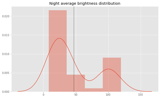



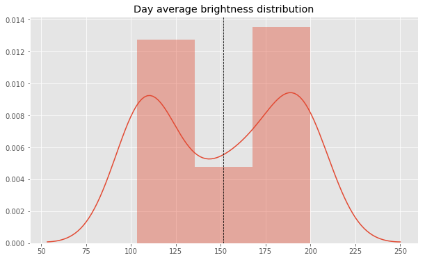
Next, our step will be to look at average brightness value for day and night images.
Our goal is to find a value (threshold), that clearly separates day and night.

Classification

Create predicted_label that will turn 1 for a day image and 0 for night image.
We will build estimate_label function that will input average brightness of an image and output an estimated label based on threshold.
Let's set threshold value = 110 for this classifier.

Next we write a class called SimpleClassifier with input:

• standardized list;
  

and output:

• accuracy;
• list of true/predicted labels.

# use RGB image as an output
def estimate_label(rgb_image):
    avg = average_brightness(rgb_image)
    predicted_label = 0
    threshold = 110
    predicted_label = 1 if avg >=threshold else predicted_label
    return predicted_label

"""
- convert to HSV colorspace
- sum up by Value
- divide resulted sum by number of pixels
"""

def average_brightness(rgb_image):
    rgb_image = np.copy(rgb_image)    
    image_hsv = cv2.cvtColor(rgb_image, cv2.COLOR_RGB2HSV)
    # add up all the pixel values in V channel
    value = np.sum(image_hsv[:,:, 2])
    # multiply height and width
    pxl = image_hsv.shape[0] * image_hsv.shape[1]
    average_value = round(value/pxl,3)
    return average_value

"""
 - Create a classifier object;
 - Recall, each item in standardized image list consists of:
   a) item[0] - image itself;
   b) item[1] - true label;
   c) item[2] - average brightness value;
   d) item[3] - predicted label.

"""
class SimpleClassifier():
    def __init__(self):
        self.predictions = []
    def predict_label(self, standardized_list, threshold):
        s1 = AverageBrightness()
        full_list = s1.average_bright(standardized_list)
        for item in full_list:
            brightness_value = item[2]
            if brightness_value >= threshold:
                # will return 1 or 0 (day or night)
                item = item + (1,)
            else:
                item = item + (0,)
            self.predictions.append((item[1], item[3]))
            # check how many labels are classified right
            confusion_list = [i[0]==i[1] for i in self.predictions]
            accuracy = sum(confusion_list) / len(confusion_list)
        return self.predictions, round(accuracy, 2)

s2 = SimpleClassifier()
estimated_labels_list = s2.predict_label(IMAGE_LIST_stand, threshold = 110)

print('Accuracy of Simple Classifier: ',estimated_labels_list[1])

Accuracy of Simple Classifier:  0.85

Testing classifier

Since we are using simple brightness as a feature, we do not expect a high accuracy for our classifier.
We aim to get 75-85% of accuracy using a single feature.

Loading the test data, we standardize and shuffle it: last ensures that the order of our data will not play a role in testing accuracy.

"""
- lead test dataset and apply standardize_input() function, that we created previously
- shuffle data using random function
"""
import random
s1 = Standardize()

TEST_IMAGE_LIST = helpers.load_dataset(image_dir_test)
TEST_IMAGE_LIST_std = s1.standardize_input(TEST_IMAGE_LIST)

random.shuffle(TEST_IMAGE_LIST_std)

Let's rewrite classifier in functional form. We will iterate through the test data images and add misclassified images and their labels into misclassified_images_lables list.

def get_misclassified_labels(test_images):
    # create an empty list, whre we will pass images and corresponding labels
    misclassified_images_lables = []
    # then we iterate through images
    # classify them and compare to the labels
    for item in test_images:
        img = item[0]
        true_label = item[1]
        # apply created function
        predicted_label = estimate_label(img)
        # compare labels and add them to misclassified_list
        if (predicted_label != true_label):
            misclassified_images_lables.append((img, predicted_label, true_label))
    return misclassified_images_lables

mis_classed_list = get_misclassified_labels(TEST_IMAGE_LIST_std)
total_images = len(TEST_IMAGE_LIST_std)
misclass = len(mis_classed_list)

print('Accuracy:', (total_images-misclass)/total_images)

Accuracy: 1.0